Tzu-Chun’s Tidy Tuesday Exercise 2

For this week’s exercise, I will continue to work on some more tidymodeling using the marble runs dataset. You can find the original data and more information in the link.

load required packages

library(here) #to set path for importing data
library(skimr)
library(readr)
library(dplyr) #for data wrangling and cleaning
library(tidymodels) # for model fitting
library(tidyverse) # data wrangling 
library(dotwhisker)  # for visualizing regression results
library(lme4) # for fitting multilevel models
library(gtsummary)
library(gt)
library(ggpubr) # for ggarrange function
library(tidymodels) #for model fitting 
library(tidyverse) #for data processing 
library(rsample) #for data splitting 
library(parsnip)
library(rpart) # for tree-based model
library(glmnet) #
library(ranger) #
library(dials) # for creating a grid of values
library(rpart.plot) # for visualizing decision tree
library(vip) # estimate variable importance based on the model’s structure
library(ggpubr) # ggarrange
library(Hmisc)
library(naniar)
library(tictoc)
library(xgboost)
library(LiblineaR)
library(finetune)
library(kableExtra)

load data

# Get the Data
marbles <- readr::read_csv('https://raw.githubusercontent.com/rfordatascience/tidytuesday/master/data/2020/2020-06-02/marbles.csv')

## 
## -- Column specification --------------------------------------------------------
## cols(
##   date = col_character(),
##   race = col_character(),
##   site = col_character(),
##   source = col_character(),
##   marble_name = col_character(),
##   team_name = col_character(),
##   time_s = col_double(),
##   pole = col_character(),
##   points = col_double(),
##   track_length_m = col_double(),
##   number_laps = col_double(),
##   avg_time_lap = col_double(),
##   host = col_character(),
##   notes = col_character()
## )

# quick descriptive information about the data
skimr::skim(marbles)

Data summary

Name	marbles
Number of rows	256
Number of columns	14
_______________________
Column type frequency:
character	9
numeric	5
________________________
Group variables	None

Variable type: character

skim_variable	n_missing	complete_rate	min	max	empty	n_unique	whitespace
date	0	1.00	8	9	0	16	0
race	0	1.00	4	4	0	16	0
site	0	1.00	7	15	0	8	0
source	0	1.00	34	34	0	16	0
marble_name	0	1.00	4	9	0	32	0
team_name	0	1.00	6	16	0	16	0
pole	128	0.50	2	3	0	16	0
host	0	1.00	2	3	0	2	0
notes	249	0.03	37	100	0	7	0

Variable type: numeric

skim_variable	n_missing	complete_rate	mean	sd	p0	p25	p50	p75	p100	hist
time_s	3	0.99	190.84	169.13	17.76	28.40	36.28	338.16	492.01	<U+2587><U+2581><U+2581><U+2587><U+2581>
points	128	0.50	6.45	7.74	0.00	0.00	3.00	11.25	26.00	<U+2587><U+2582><U+2582><U+2581><U+2581>
track_length_m	0	1.00	13.22	0.95	11.90	12.62	13.02	14.13	14.55	<U+2585><U+2585><U+2582><U+2581><U+2587>
number_laps	0	1.00	6.25	5.53	1.00	1.00	5.00	10.25	16.00	<U+2587><U+2581><U+2583><U+2582><U+2582>
avg_time_lap	3	0.99	29.70	5.55	17.76	25.94	30.05	33.65	41.62	<U+2583><U+2586><U+2587><U+2587><U+2582>

First, let’s explore the dataset by looking at the

data exploration

# check data structure
glimpse(marbles)

## Rows: 256
## Columns: 14
## $ date           <chr> "15-Feb-20", "15-Feb-20", "15-Feb-20", "15-Feb-20", "15~
## $ race           <chr> "S1Q1", "S1Q1", "S1Q1", "S1Q1", "S1Q1", "S1Q1", "S1Q1",~
## $ site           <chr> "Savage Speedway", "Savage Speedway", "Savage Speedway"~
## $ source         <chr> "https://youtu.be/JtsQ_UydjEI?t=356", "https://youtu.be~
## $ marble_name    <chr> "Clementin", "Starry", "Momo", "Yellow", "Snowy", "Razz~
## $ team_name      <chr> "O'rangers", "Team Galactic", "Team Momo", "Mellow Yell~
## $ time_s         <dbl> 28.11, 28.37, 28.40, 28.70, 28.71, 28.72, 28.96, 29.11,~
## $ pole           <chr> "P1", "P2", "P3", "P4", "P5", "P6", "P7", "P8", "P9", "~
## $ points         <dbl> NA, NA, NA, NA, NA, NA, NA, NA, NA, NA, NA, NA, NA, NA,~
## $ track_length_m <dbl> 12.81, 12.81, 12.81, 12.81, 12.81, 12.81, 12.81, 12.81,~
## $ number_laps    <dbl> 1, 1, 1, 1, 1, 1, 1, 1, 1, 1, 1, 1, 1, 1, 1, 1, 10, 10,~
## $ avg_time_lap   <dbl> 28.11, 28.37, 28.40, 28.70, 28.71, 28.72, 28.96, 29.11,~
## $ host           <chr> "No", "No", "No", "No", "No", "No", "No", "No", "No", "~
## $ notes          <chr> NA, NA, NA, NA, NA, NA, NA, NA, NA, NA, NA, NA, NA, NA,~

# descriptive summary table  
marbles %>% 
# select only important variables
  select(2,3,5:13) %>% 
  tbl_summary() %>% 
  modify_header(label ~ "**Variable**") %>% 
  bold_labels()  %>%
  as_flex_table()

Variable	N = 2561
race
S1Q1	16 (6.2%)
S1Q2	16 (6.2%)
S1Q3	16 (6.2%)
S1Q4	16 (6.2%)
S1Q5	16 (6.2%)
S1Q6	16 (6.2%)
S1Q7	16 (6.2%)
S1Q8	16 (6.2%)
S1R1	16 (6.2%)
S1R2	16 (6.2%)
S1R3	16 (6.2%)
S1R4	16 (6.2%)
S1R5	16 (6.2%)
S1R6	16 (6.2%)
S1R7	16 (6.2%)
S1R8	16 (6.2%)
site
Greenstone	32 (12%)
Hivedrive	32 (12%)
Midnight Bay	32 (12%)
Momotorway	32 (12%)
O'raceway	32 (12%)
Razzway	32 (12%)
Savage Speedway	32 (12%)
Short Circuit	32 (12%)
marble_name
Anarchy	8 (3.1%)
Billy	8 (3.1%)
Bolt	8 (3.1%)
Clementin	8 (3.1%)
Clutter	8 (3.1%)
Hazy	8 (3.1%)
Hive	8 (3.1%)
Limelime	8 (3.1%)
Mallard	8 (3.1%)
Mary	8 (3.1%)
Mimo	8 (3.1%)
Momo	8 (3.1%)
Orangin	8 (3.1%)
Prim	8 (3.1%)
Pulsar	8 (3.1%)
Rapidly	8 (3.1%)
Razzy	8 (3.1%)
Rezzy	8 (3.1%)
Rojo Dos	8 (3.1%)
Rojo Uno	8 (3.1%)
Shock	8 (3.1%)
Smoggy	8 (3.1%)
Snowflake	8 (3.1%)
Snowy	8 (3.1%)
Speedy	8 (3.1%)
Starry	8 (3.1%)
Sublime	8 (3.1%)
Vespa	8 (3.1%)
Wispy	8 (3.1%)
Wospy	8 (3.1%)
Yellow	8 (3.1%)
Yellup	8 (3.1%)
team_name
Balls of Chaos	16 (6.2%)
Green Ducks	16 (6.2%)
Hazers	16 (6.2%)
Hornets	16 (6.2%)
Limers	16 (6.2%)
Mellow Yellow	16 (6.2%)
Midnight Wisps	16 (6.2%)
O'rangers	16 (6.2%)
Raspberry Racers	16 (6.2%)
Rojo Rollers	16 (6.2%)
Savage Speeders	16 (6.2%)
Snowballs	16 (6.2%)
Team Galactic	16 (6.2%)
Team Momo	16 (6.2%)
Team Primary	16 (6.2%)
Thunderbolts	16 (6.2%)
time_s	36 (28, 338)
Unknown	3
pole
P1	8 (6.2%)
P10	8 (6.2%)
P11	8 (6.2%)
P12	8 (6.2%)
P13	8 (6.2%)
P14	8 (6.2%)
P15	8 (6.2%)
P16	8 (6.2%)
P2	8 (6.2%)
P3	8 (6.2%)
P4	8 (6.2%)
P5	8 (6.2%)
P6	8 (6.2%)
P7	8 (6.2%)
P8	8 (6.2%)
P9	8 (6.2%)
Unknown	128
points	3 (0, 11)
Unknown	128
track_length_m
11.9	32 (12%)
12.05	32 (12%)
12.81	32 (12%)
12.84	32 (12%)
13.2	32 (12%)
14.05	32 (12%)
14.38	32 (12%)
14.55	32 (12%)
number_laps
1	128 (50%)
9	32 (12%)
10	32 (12%)
11	16 (6.2%)
13	16 (6.2%)
14	16 (6.2%)
16	16 (6.2%)
avg_time_lap	30 (26, 34)
Unknown	3
host	16 (6.2%)
1n (%); Median (IQR)

There are 16 races, 8 sites, 32 marble names, 16 teams, 17 different pole positions, 8 different track lengths. Next, I want to examine whether the missing data varies by race sites.

Examine missing data

# check percentage of missing values in each column by flu season
aggregate(marbles , by=list(marbles$site), FUN = function(x) { sum(is.na(x))/length(x)*100 })

##           Group.1 date race site source marble_name team_name time_s pole
## 1      Greenstone    0    0    0      0           0         0  0.000   50
## 2       Hivedrive    0    0    0      0           0         0  3.125   50
## 3    Midnight Bay    0    0    0      0           0         0  0.000   50
## 4      Momotorway    0    0    0      0           0         0  0.000   50
## 5       O'raceway    0    0    0      0           0         0  3.125   50
## 6         Razzway    0    0    0      0           0         0  0.000   50
## 7 Savage Speedway    0    0    0      0           0         0  0.000   50
## 8   Short Circuit    0    0    0      0           0         0  3.125   50
##   points track_length_m number_laps avg_time_lap host   notes
## 1     50              0           0        0.000    0 100.000
## 2     50              0           0        3.125    0 100.000
## 3     50              0           0        0.000    0  93.750
## 4     50              0           0        0.000    0 100.000
## 5     50              0           0        3.125    0 100.000
## 6     50              0           0        0.000    0  87.500
## 7     50              0           0        0.000    0 100.000
## 8     50              0           0        3.125    0  96.875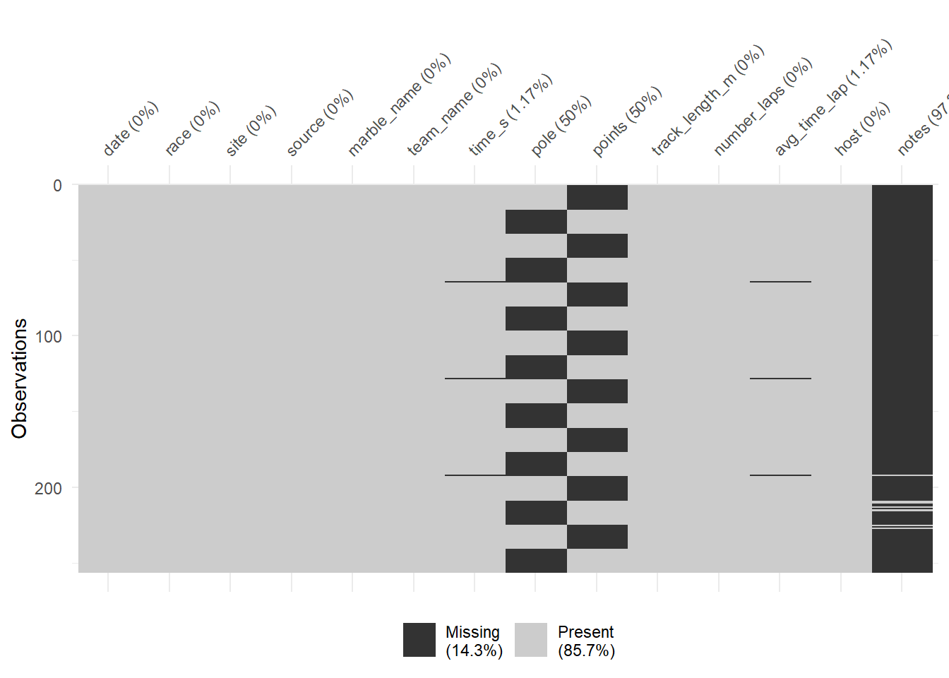

vis_miss(marbles)

It looks like pole positions and points gained had 50% data missing, and there are some missingness in time in seconds and average lap time. In addition, the last two information were only missing in three sites.

Data processing

For further analysis, I will remove missing data since there are only less than 10% missing. Both variables, pole and points will be drop from the analysis due to substantial missing data. Let’s clean up the data now!

marbles.clean <- 
marbles %>%
  # exclude variables that will not be included for analysis as well
  select(-date, -source, -pole, -points, -notes) %>% 
  drop_na(time_s, avg_time_lap)

In Randy’s blogpost, he mentioned that he had to standardize the race times since each race track took a varying amount of time. I will also standardize the data using the same approach. First, I will calculate the average race time for different race and divide individual marble’s time by the average. This way, we will get the standardized performance in each race for each marble, checking how better or worse the marble performed compared to that race track.

marbles.clean <- 
  marbles.clean %>% 
  group_by(race) %>% 
  # average race time for each race
  mutate(average_race_time = mean(time_s)) %>% 
  ungroup() %>% 
  # marble's race time relative to average race time
  mutate(std_time = time_s/average_race_time) 

More exploratory data analysis

# plotting for the continuous outcome, std_time 
marbles.clean %>% 
ggplot(aes(x=std_time)) + 
  geom_histogram(bins = 100) +
  xlab("Standardized race time for individual marble relative to average race time") +
  ylab("Frequency") +
  ggtitle("Histogram of standardized race time") +
  theme_bw()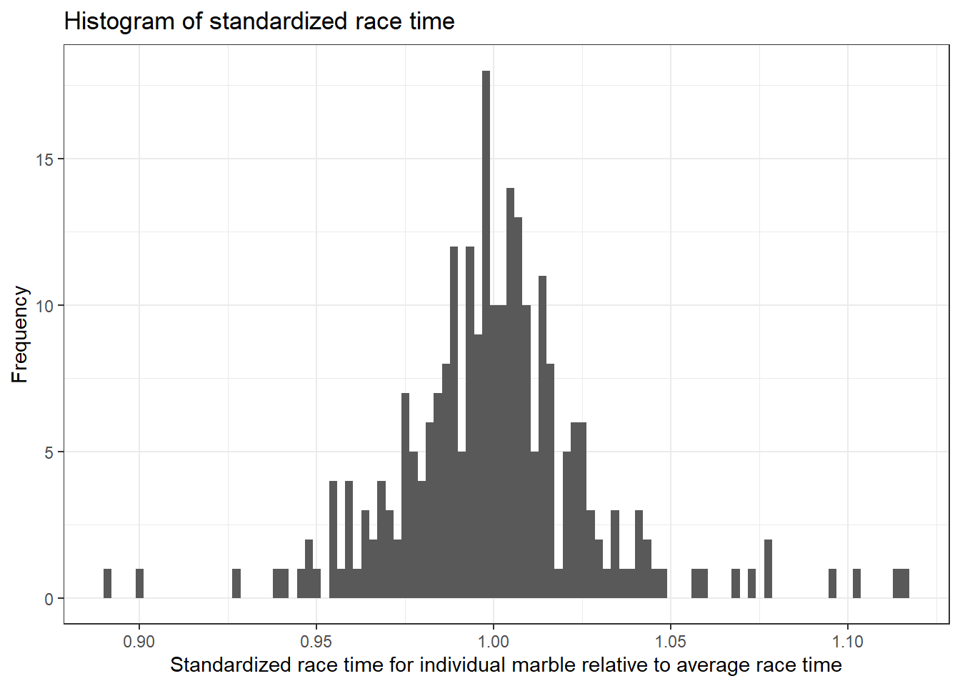

We can see that the standardized race time for each marble follows a normal distribution.

Next, I want to know which team performed the best, and whether specific marble ran faster.

# boxplot of standardized race time by track team
marbles.clean %>% 
  ggplot(aes(x=team_name, y=std_time)) + 
    geom_boxplot() +
    xlab("") +
    ylab("Standardized race time") +
    theme(axis.text.x = element_text(angle = 45, hjust=1)) +
    ggtitle("Boxplot of standardized race time by track team")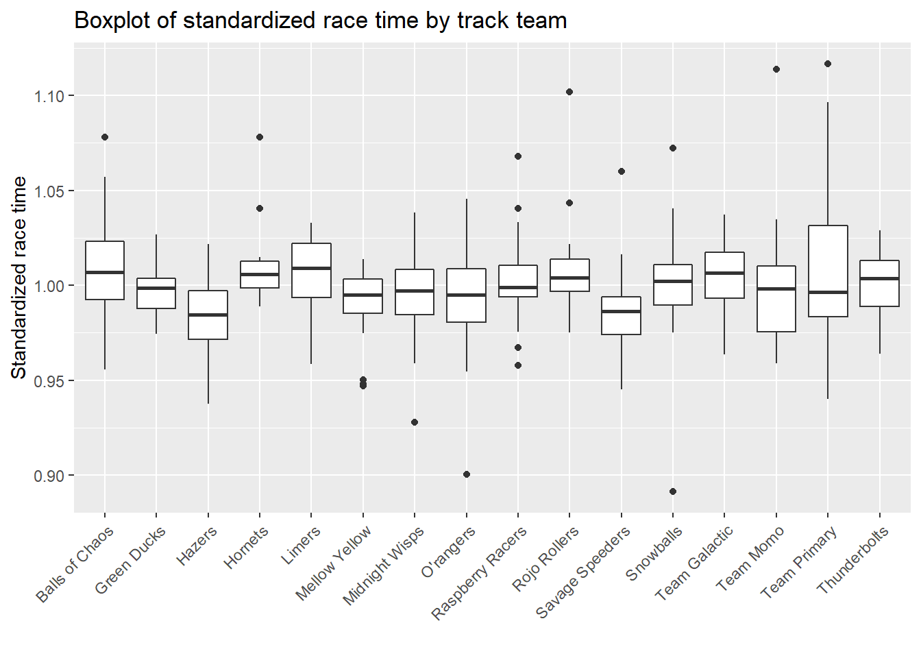

# boxplot of standardized race time by marble
marbles.clean %>% 
  ggplot(aes(x=marble_name, y=std_time)) + 
    geom_boxplot() +
    xlab("") +
    ylab("Standardized race time") +
    theme(axis.text.x = element_text(angle = 45, hjust=1)) +
    ggtitle("Boxplot of standardized race time by marble")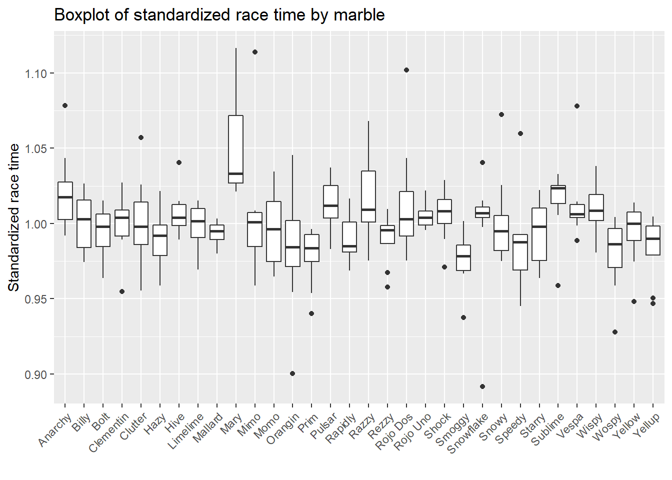

ML data modeling

The main outcome of interest is the standardized race time, and we will fit six candidate predictors in four different ML models to determine their predictive ability. Next, I will create outcome and predictor variables needed for modeling.

# create variables for modeling
marbles.final <-
  marbles.clean %>% 
  transmute(
    race   = factor(race),
    marble = factor(marble_name),
    team   = factor(team_name),
    host   = factor(host),
    track_length_m = as.numeric(track_length_m),
    number_laps = as.numeric(std_time),
    std_time = as.numeric(std_time)
  )

Data setup

# Data Splitting------------------------------------------------------
#set seed to fix random numbers 
set.seed(123)

# put 0.7 of data into training set, use BodyTemp as stratification
data_split <- initial_split( marbles.final, 
                                                        prop = 0.7,
                                                        strata = std_time)

# create data frames for training and testing sets 
train_data <- training(data_split)
test_data <- testing(data_split)

# create 5-fold cross-validation, 5 times repeated
folds <- vfold_cv(train_data, v = 5, repeats =5, strata = std_time)

# create recipe fitting BodyTemp to all predictors 
rec <- recipes::recipe(std_time ~ ., data = train_data)

# create dummy variable for all predictors
rec_all_pred <- rec %>%
    #converts characters or factors 
  step_dummy(all_nominal()) %>%
    #removes indicator variables that only contain a single unique value
  step_zv(all_predictors())

Model tuning and fitting

Decision tree

I first followed the tidymodels tutorial for training the model using tree regression method, but I got the error of the "“a correlation computation is required, but ‘estimate’ is constant and has…” when I used dials to search for all tuning combinations to try for each hyperparameter, and the final tree didn’t perform well, and only include sneeze as only predictor. I would like to thank Zane for the inspiration, I used “grid_latin_hypercube” for defining a grid of potential parameter values, and the codes ran without any error.

# model specification 
tree_spec <- 
  decision_tree(
    cost_complexity = tune(),
    tree_depth = tune(),
    min_n = tune() # sets the minimum n to split at any node.
  ) %>% 
  set_engine("rpart") %>% 
  set_mode("regression")

tree_spec

## Decision Tree Model Specification (regression)
## 
## Main Arguments:
##   cost_complexity = tune()
##   tree_depth = tune()
##   min_n = tune()
## 
## Computational engine: rpart

# we will train this specification on several re-sampled data
tree_wf <- workflow() %>% 
  add_model(tree_spec) %>% 
  add_recipe(rec_all_pred)


# define a grid of potential parameter values using latin hypercube sampling
tree_grid <- grid_latin_hypercube(
  cost_complexity(), tree_depth(), min_n(), size = 10
)

# Grid search for parameter values
tree_res <- tree_wf %>% 
  tune_grid(
    resamples = folds,
    grid = tree_grid,
    metrics = metric_set(rmse),
    control = control_grid(verbose = TRUE),
 )


# Select single set of hyperparameter values for our best decision tree model
best_tree <- select_best(tree_res)

# Finalize our workflow with best values
final_tree_wf <- tree_wf %>% 
  finalize_workflow(best_tree)

# Fit model to training data
best_tree_train_fit <- final_tree_wf %>%  
    fit(data = train_data)


png(filename = here::here("tidytuesday2_figures", "tree_algorithms.png"), width = 1200, height = 1000)

rpart.plot::rpart.plot(
  x = extract_fit_parsnip(best_tree_train_fit)$fit,
  main = "Final tree-based model",
  roundint = F,
  type = 5,
  digits = 4
)
dev.off()

## png 
##   2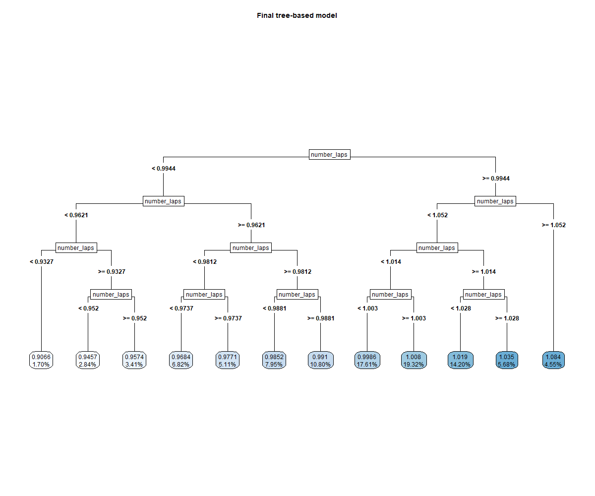

knitr::include_graphics( here::here("tidytuesday2_figures", "tree_algorithms.png"))

# estimate model importance based on the model's structure
vip_tree <-
best_tree_train_fit %>% 
  extract_fit_parsnip() %>% 
  vip()

vip_tree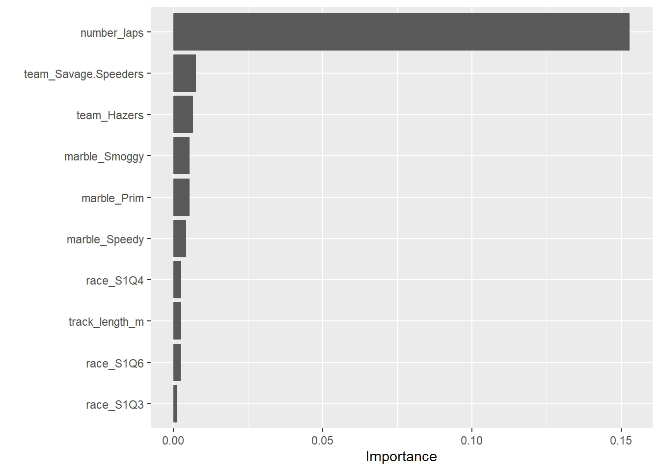

Number of laps is the strongest predictor of the race time.

Diagnostics plots

# some more diagnostics
tree_diagnostics <- 
  tree_res %>% autoplot()

ggsave(filename = here::here("tidytuesday2_figures", "tree_diagnostics.png"),
       plot = tree_diagnostics,
       width = 12, height = 6)

knitr::include_graphics( here::here("tidytuesday2_figures", "tree_diagnostics.png"))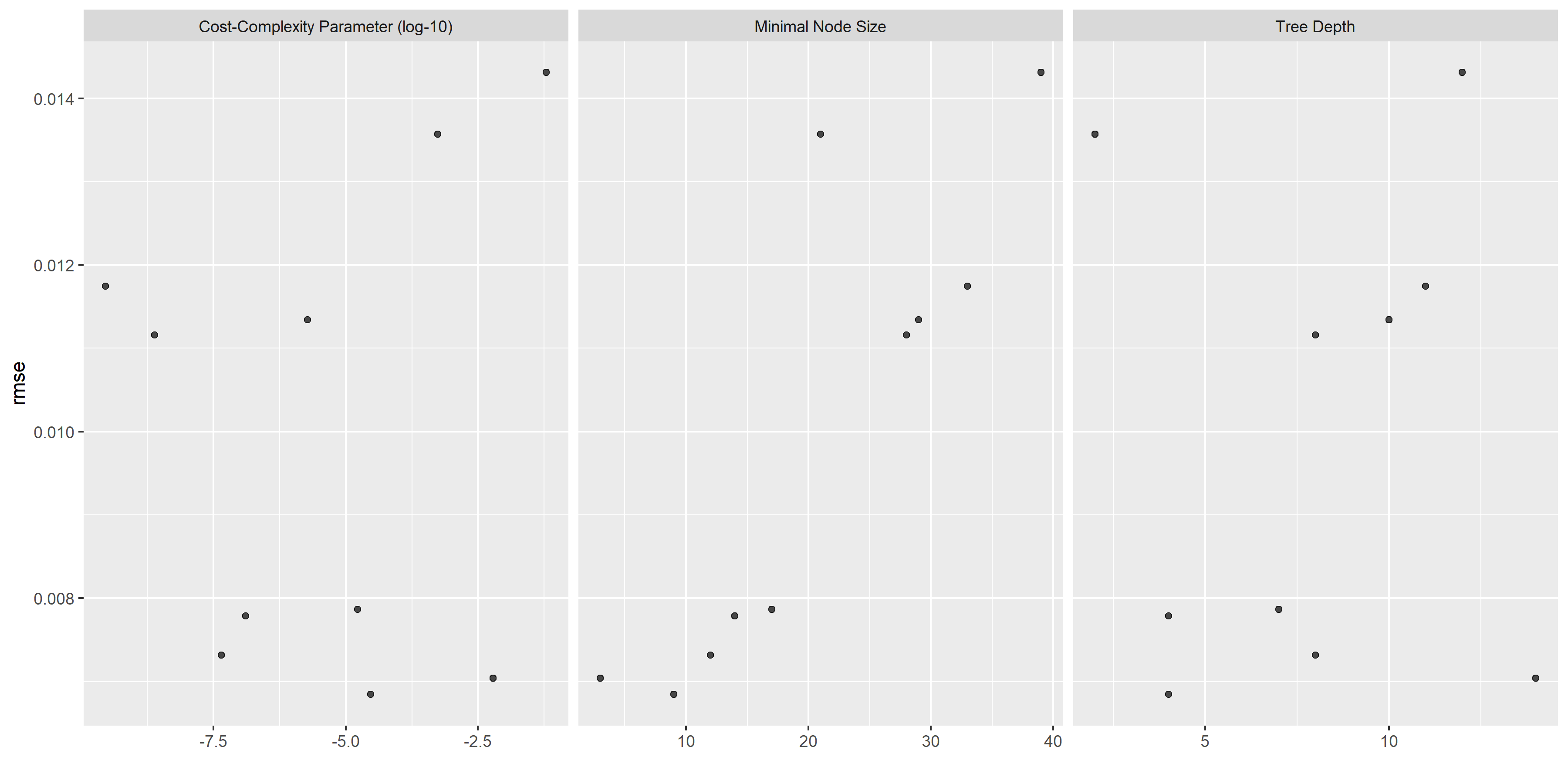

# pull predictions and residuals
tree_train_res <- best_tree_train_fit  %>% 
  augment(new_data = train_data) %>% 
         select(.pred, std_time) %>% 
         mutate(.resid = std_time - .pred)


# plot Predictions vs observed values
p1 <- ggplot(tree_train_res, aes(x = std_time, y = .pred)) +
  geom_abline(slope = 1, intercept = 0, color = "red", lty = 2) +
  geom_point() +
  cowplot::theme_cowplot() +
  labs(
    title = "Decision tree: predicted vs observed",
    x = "Observed",
    y = "Fitted"
  )

# Plot model predictions vs residuals
p2 <- ggplot(tree_train_res, aes(y = .resid, x = .pred)) +
  geom_hline(yintercept = 0, color = "red", lty = 2) +
  geom_point() +
  cowplot::theme_cowplot() +
  labs(
    title = "Decision tree: residuals vs fitted",
    y = "Residuals",
    x = "Fitted"
  )

# combine graphs
tree_panel <- cowplot::plot_grid(p1, p2, labels = c('A', 'B'), label_size = 12, ncol =2)

ggsave(filename = here::here("tidytuesday2_figures", "tree_panel.png"),
       plot = tree_panel,
       width = 12, height = 6)

knitr::include_graphics( here::here("tidytuesday2_figures", "tree_panel.png"))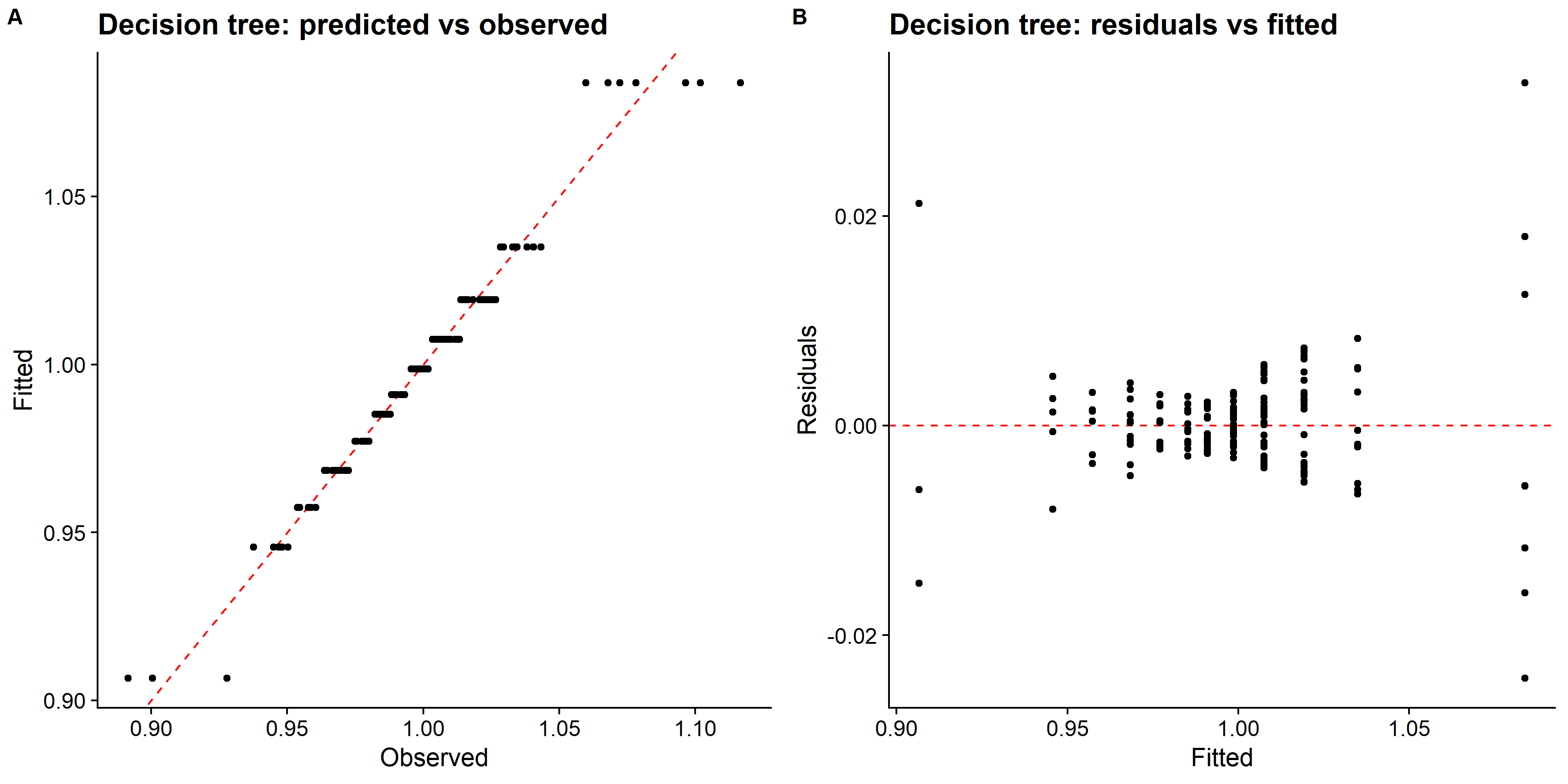

# looking at model performance
tree_perfomance <- tree_res %>% show_best(n = 1)
print(tree_perfomance) # rmse: 0.0068

## # A tibble: 1 x 9
##   cost_complexity tree_depth min_n .metric .estimator    mean     n  std_err
##             <dbl>      <int> <int> <chr>   <chr>        <dbl> <int>    <dbl>
## 1       0.0000297          4     9 rmse    standard   0.00685    25 0.000517
## # ... with 1 more variable: .config <chr>

The RMSE of the regression tree model is small and the predicted vs observed plot looks good. All the data points seem to align with the diagonal line.

LASSO model

# LASSO model specification 
lasso_spec <- 
  linear_reg(
    penalty = tune(),
    mixture = 1 # make this LASSO
  ) %>% 
  set_engine("glmnet") %>% 
  set_mode("regression")

lasso_spec

## Linear Regression Model Specification (regression)
## 
## Main Arguments:
##   penalty = tune()
##   mixture = 1
## 
## Computational engine: glmnet

lasso_wf <- workflow() %>% 
  add_model(lasso_spec) %>% 
  add_recipe(rec_all_pred)

# only one hyperparameter to tune here, we can set the grid up manually using a one-column # tibble with 30 candidate values
lasso_grid <- tibble(penalty = 10^seq(-4, -1, length.out = 30))

# use grid search to tune hyperparameters using cross-validation 
lasso_res <- lasso_wf %>% 
  tune::tune_grid(
    resamples = folds,
    grid = lasso_grid,
    metrics =  metric_set(rmse),
    control = control_grid(verbose = TRUE)
  )

# pull the best tuning parameter values
best_lasso <- select_best(lasso_res)

# Finalize workflow with best values
final_lasso_wf <- lasso_wf  %>% 
  finalize_workflow(best_lasso)

# Fit model to training data
best_lasso_train_fit <- final_lasso_wf %>%  fit(data = train_data)

Diagnostics plots

# LASSO variable trace plot
x <- best_lasso_train_fit$fit$fit$fit
plot(x, "lambda")

## Warning in plotCoef(x$beta, lambda = x$lambda, df = x$df, dev = x$dev.ratio, : 1
## or less nonzero coefficients; glmnet plot is not meaningful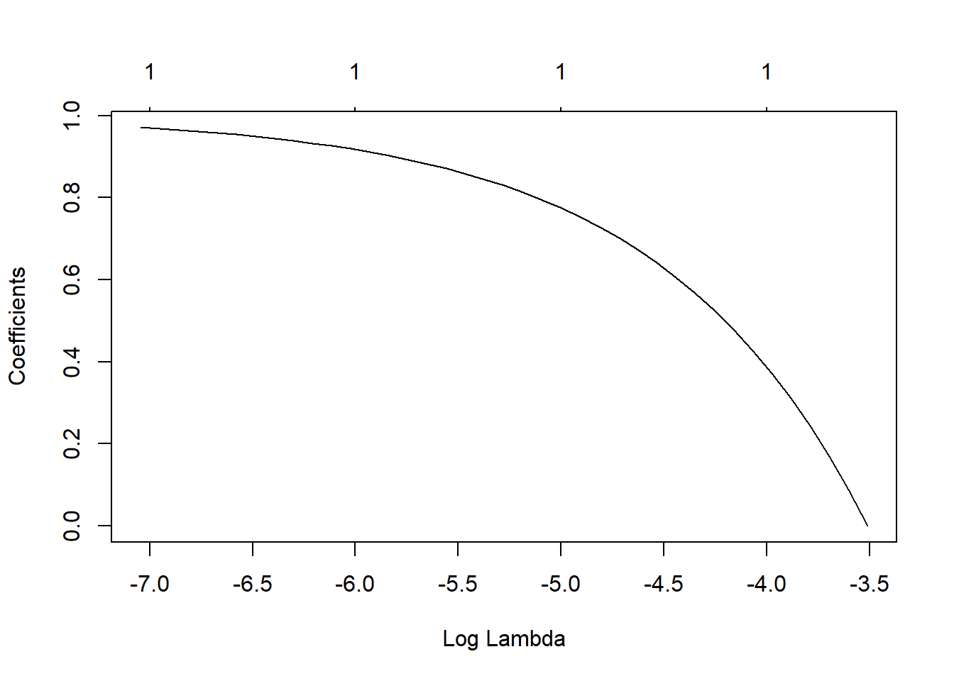

More diagnostics plots

# some more diagnostics
lasso_diagnostics <- 
lasso_res %>% autoplot()

ggsave(filename = here::here("tidytuesday2_figures", "lasso_diagnostics.png"),
       plot = lasso_diagnostics,
       width = 12, height = 6)

knitr::include_graphics( here::here("tidytuesday2_figures", "lasso_diagnostics.png"))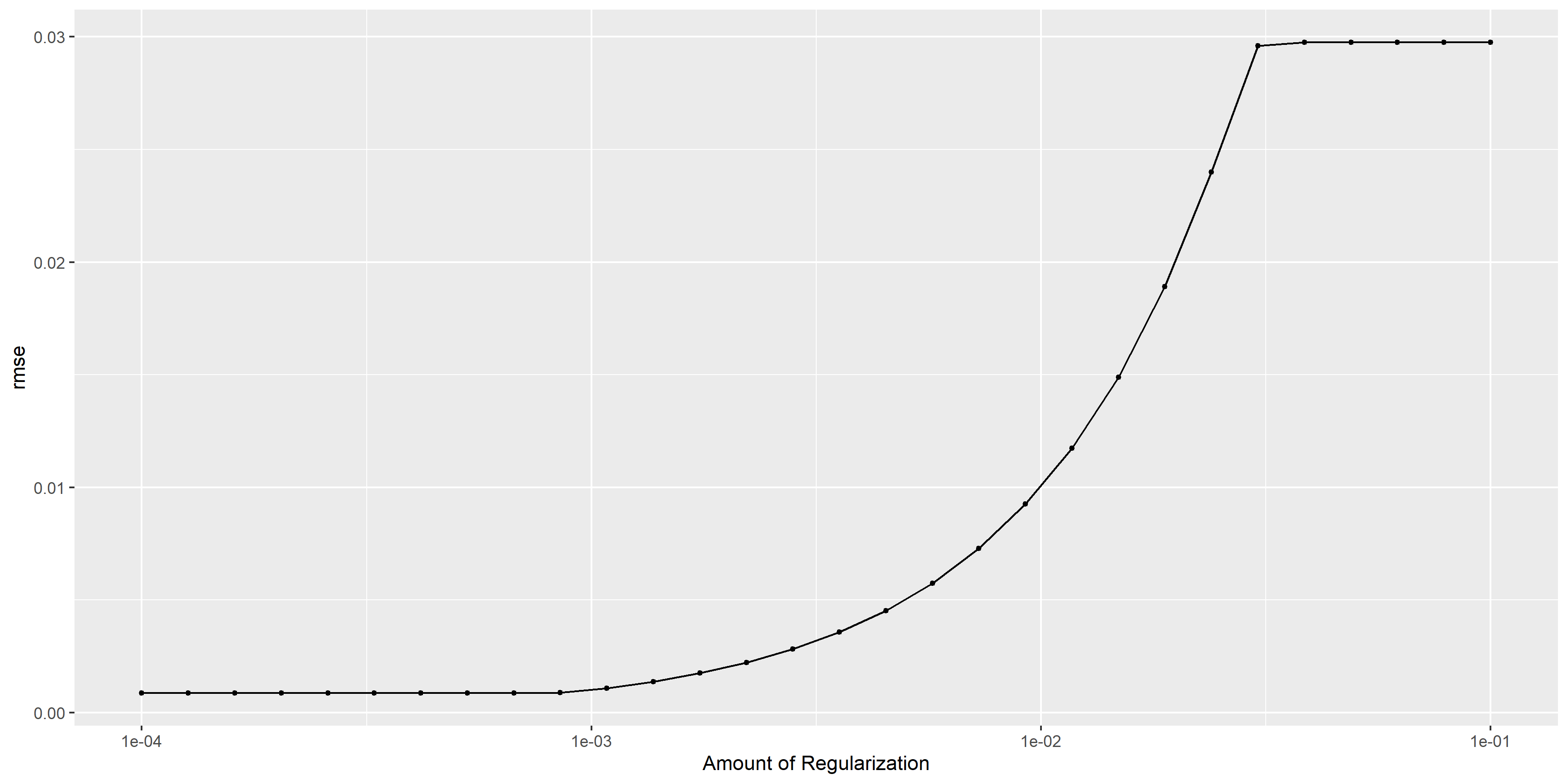

# pull predictions and residuals
lasso_train_res <- best_lasso_train_fit  %>% 
  augment(new_data = train_data) %>% 
         select(.pred, std_time) %>% 
         mutate(.resid = std_time - .pred)


# plot Predictions vs observed values
p1 <- ggplot(lasso_train_res, aes(x = std_time, y = .pred)) +
  geom_abline(slope = 1, intercept = 0, color = "red", lty = 2) +
  geom_point() +
  cowplot::theme_cowplot() +
  labs(
    title = "LASSO: predicted vs observed",
    x = "Observed",
    y = "Fitted"
  )

# Plot model predictions vs residuals
p2 <- ggplot(lasso_train_res, aes(y = .resid, x = .pred)) +
  geom_hline(yintercept = 0, color = "red", lty = 2) +
  geom_point() +
  cowplot::theme_cowplot() +
  labs(
    title = "LASSO: residuals vs fitted",
    y = "Residuals",
    x = "Fitted"
  )

# combine graphs
lasso_panel <- cowplot::plot_grid(p1, p2, labels = c('A', 'B'), label_size = 12, ncol =2)

ggsave(filename = here::here("tidytuesday2_figures", "lasso_panel.png"),
       plot = lasso_panel,
       width = 12, height = 6)

knitr::include_graphics( here::here("tidytuesday2_figures", "lasso_panel.png"))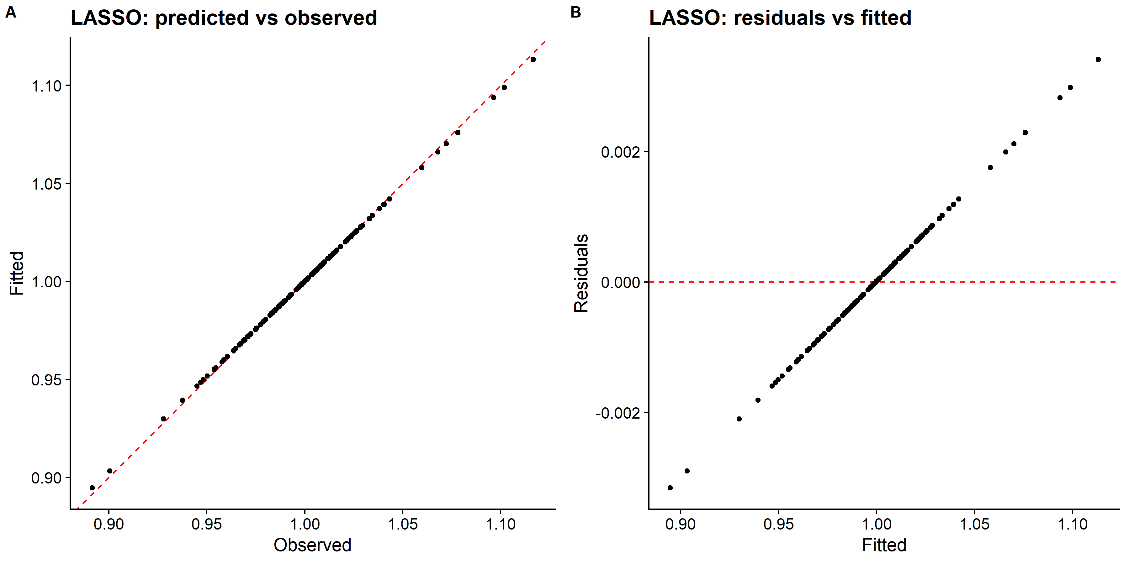

# looking at model performance
lasso_perfomance <- lasso_res %>% show_best(n = 1)
print(lasso_perfomance) # rmse: 0.0008

## # A tibble: 1 x 7
##   penalty .metric .estimator     mean     n   std_err .config              
##     <dbl> <chr>   <chr>         <dbl> <int>     <dbl> <chr>                
## 1  0.0001 rmse    standard   0.000867    25 0.0000252 Preprocessor1_Model01

The RMSE is smaller compared to the single tree model, however the residual plot looks weird.

Random forrest

# query number of cores and see how much paralleization that can be done
cores <- parallel::detectCores()
cores # 4

## [1] 4

# pass information to ranger engine to set up the model
rf_mod <- 
  rand_forest(mtry = tune(), min_n = tune(), trees = 1000) %>% 
  set_engine("ranger", num.threads = cores, importance = "permutation") %>% 
  set_mode("regression")

# create workflow to bundle model spec and recipe
rf_wf <- workflow() %>% 
  add_model(rf_mod) %>% 
  add_recipe(rec_all_pred)

# show what will be tuned
rf_mod %>%    
  parameters()  

## Collection of 2 parameters for tuning
## 
##  identifier  type    object
##        mtry  mtry nparam[?]
##       min_n min_n nparam[+]
## 
## Model parameters needing finalization:
##    # Randomly Selected Predictors ('mtry')
## 
## See `?dials::finalize` or `?dials::update.parameters` for more information.

# use a space-filling design to tune, with 25 candidate models
rf_res <- 
  rf_wf %>% 
  tune_grid(folds,
            grid = 25,
            control = control_grid(save_pred = TRUE),
            metrics = metric_set(rmse))

# 5 random forest models, out of the 25 candidates:
rf_res %>% 
  show_best(metric = "rmse")

## # A tibble: 5 x 8
##    mtry min_n .metric .estimator    mean     n  std_err .config              
##   <int> <int> <chr>   <chr>        <dbl> <int>    <dbl> <chr>                
## 1    63     8 rmse    standard   0.00520    25 0.000515 Preprocessor1_Model09
## 2    61    10 rmse    standard   0.00563    25 0.000540 Preprocessor1_Model10
## 3    57    15 rmse    standard   0.00651    25 0.000593 Preprocessor1_Model08
## 4    49    17 rmse    standard   0.00756    25 0.000659 Preprocessor1_Model17
## 5    45    13 rmse    standard   0.00763    25 0.000656 Preprocessor1_Model24

# select the best model according to RMSE metric, and the final tuning parameter values are:
best_rf <- 
  rf_res %>% 
  select_best(metric = "rmse")

best_rf

## # A tibble: 1 x 3
##    mtry min_n .config              
##   <int> <int> <chr>                
## 1    63     8 Preprocessor1_Model09

# Finalize workflow with best values
final_rf_wf <- rf_wf  %>% 
  finalize_workflow(best_rf)

# Fit model to training data
best_rf_train_fit <- final_rf_wf %>%  fit(data = train_data)

# estimate model importance based on the model's structure
vip_rf <-
best_rf_train_fit %>% 
  extract_fit_parsnip() %>% 
  vip()

vip_tree

Number of laps is the strongest predictor.

Diagnostics plots

# some more diagnostics
rf_diagnostics <- 
rf_res %>% autoplot()
ggsave(filename = here::here("tidytuesday2_figures", "random_forest_diagnostics.png"),
       plot = rf_diagnostics,
       width = 12, height = 6)

knitr::include_graphics( here::here("tidytuesday2_figures", "random_forest_diagnostics.png"))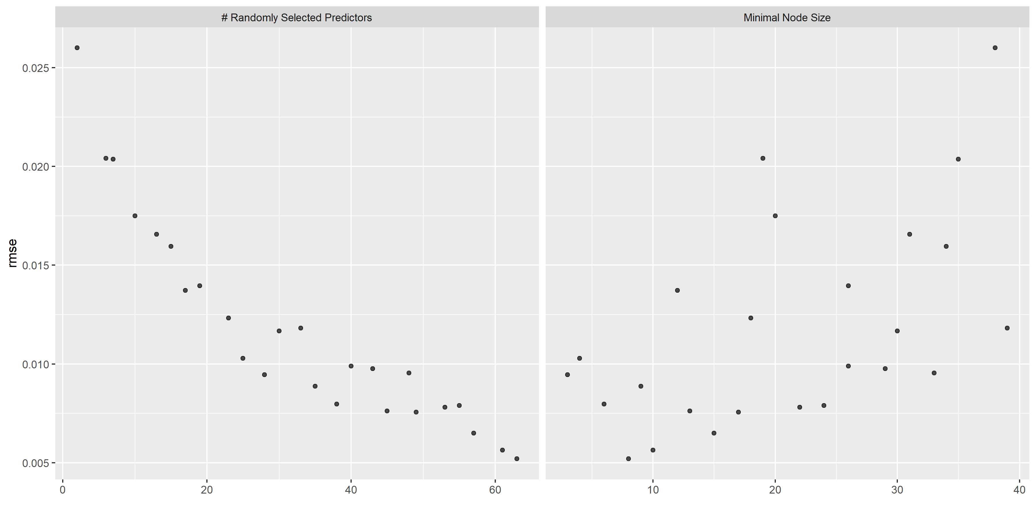

# pull predictions and residuals
rf_train_res <- best_rf_train_fit  %>% 
  augment(new_data = train_data) %>% 
         select(.pred, std_time) %>% 
         mutate(.resid = std_time - .pred)


# plot Predictions vs observed values
p1 <- ggplot(rf_train_res, aes(x = std_time, y = .pred)) +
  geom_abline(slope = 1, intercept = 0, color = "red", lty = 2) +
  geom_point() +
  cowplot::theme_cowplot() +
  labs(
    title = "Random forest: predicted vs observed",
    x = "Observed",
    y = "Fitted"
  )

# Plot model predictions vs residuals
p2 <- ggplot(rf_train_res, aes(y = .resid, x = .pred)) +
  geom_hline(yintercept = 0, color = "red", lty = 2) +
  geom_point() +
  cowplot::theme_cowplot() +
  labs(
    title = "Random forest: residuals vs fitted",
    y = "Residuals",
    x = "Fitted"
  )

# combine graphs
random_forest_panel <- cowplot::plot_grid(p1, p2, labels = c('A', 'B'), label_size = 12, ncol =2)

ggsave(filename = here::here("tidytuesday2_figures", "random_forest_panel.png"),
       plot = random_forest_panel,
       width = 12, height = 6)

knitr::include_graphics( here::here("tidytuesday2_figures", "random_forest_panel.png"))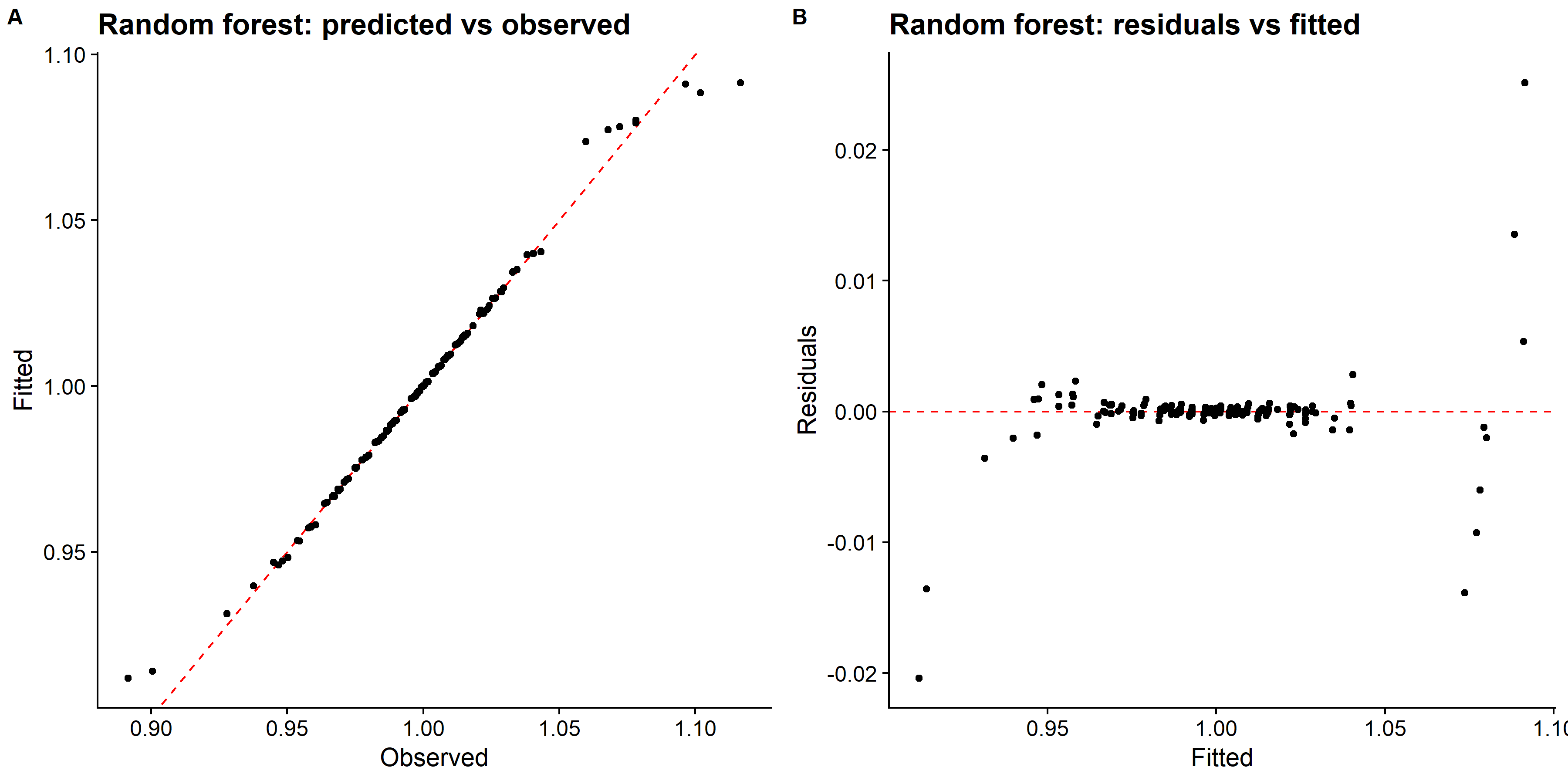

# looking at model performance
rf_perfomance <- rf_res %>% show_best(n = 1)
print(rf_perfomance) # rmse: 0.0059

## # A tibble: 1 x 8
##    mtry min_n .metric .estimator    mean     n  std_err .config              
##   <int> <int> <chr>   <chr>        <dbl> <int>    <dbl> <chr>                
## 1    63     8 rmse    standard   0.00520    25 0.000515 Preprocessor1_Model09

The RMSE is larger than LASSO model but smaller than the tree regression model. The predicted vs observed and residual plots look good.

Support vector machines

# model specification 
svm_spec <- 
  svm_linear(  
  cost = tune(), 
  margin = tune()) %>% 
  set_engine("LiblineaR") %>% 
  set_mode("regression") 


# create workflow to bundle model spec and recipe
svm_wf <- workflow() %>% 
  add_model(svm_spec) %>% 
  add_recipe(rec_all_pred)

SVM tuning

fix issue with parallel computing back-end for dopar

unregister_dopar <- function() {
  env <- foreach:::.foreachGlobals
  rm(list=ls(name=env), pos=env)
}

# parallel computing
doParallel::registerDoParallel()

# # bootstrapping 
# set.seed(123)
# iono_rs <- bootstraps(train_data, times = 30)

# finalize the parameter ranges before optimizing 
svm_parms <- svm_spec  %>%
  dials::parameters() %>%
  dials::finalize(train_data %>%  select(-titerincrease))

# Optimization of model parameters via simulated annealing
svm_res <- svm_wf %>%
  tune_sim_anneal(
    resamples = folds,
    metrics = metric_set(rmse),
    control = control_sim_anneal(
      verbose = TRUE,
      no_improve = 10,
      radius = c(0.01, 0.25),
      cooling_coef = 0.01
    ),
    iter = 10,
    param_info = svm_parms
  )

## 

## >  Generating a set of 1 initial parameter results

## v Initialization complete

## 

## Optimizing rmse

## Initial best: 0.09487

##  1 <3 new best           rmse=0.093905   (+/-0.003484)

##  2 ( ) accept suboptimal  rmse=0.10092   (+/-0.00391)

##  3 <3 new best           rmse=0.089384   (+/-0.003136)

##  4 - discard suboptimal rmse=0.10895 (+/-0.004231)

##  5 <3 new best           rmse=0.084611   (+/-0.00166)

##  6 ( ) accept suboptimal  rmse=0.085066  (+/-0.002311)

##  7 ( ) accept suboptimal  rmse=0.085751  (+/-0.002535)

##  8 ( ) accept suboptimal  rmse=0.087062  (+/-0.002753)

##  9 + better suboptimal  rmse=0.086179    (+/-0.002611)

## 10 - discard suboptimal rmse=0.10655 (+/-0.004151)

# turn off parallel cluster
doParallel::stopImplicitCluster()
unregister_dopar()
# stopCluster(cl)

Look up model performance during tuning

# plot of performance for different tuning parameters
svm_diagnostics <- svm_res %>% autoplot()

ggsave(filename = here::here("tidytuesday2_figures", "svm_diagnostics.png"),
       plot = svm_diagnostics,
       width = 12, height = 6)
knitr::include_graphics( here::here("tidytuesday2_figures", "svm_diagnostics.png"))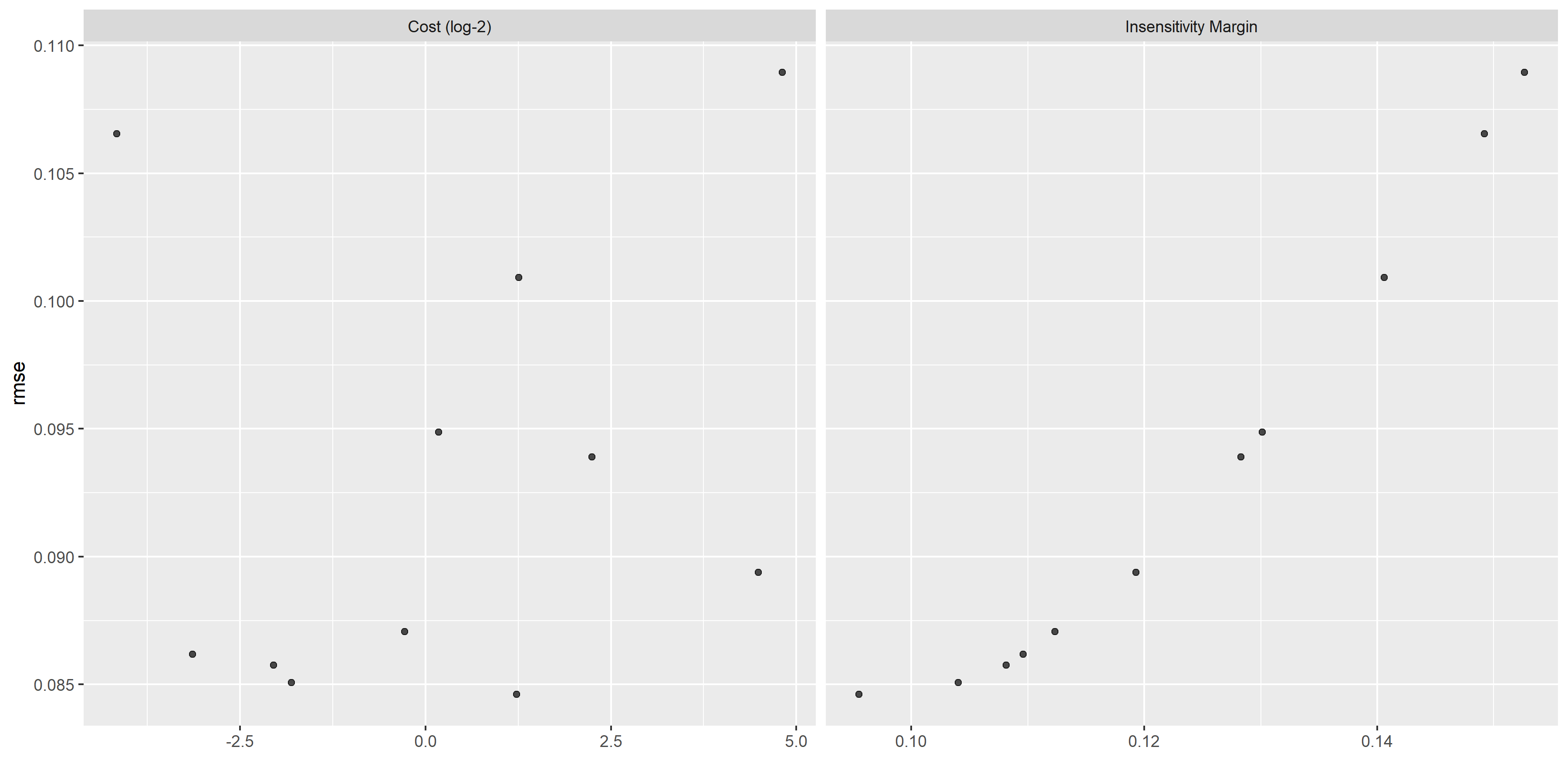

SVM model evaluation

# Select single set of hyperparameter values for our best decision tree model
best_svm <- svm_res %>%  
    select_best(metric = "rmse")

# Finalize our workflow with best values
final_svm_wf <- svm_wf %>% 
  finalize_workflow(best_svm)

# Fit model to training data
best_svm_fit_train <- final_svm_wf %>%  
    fit(data = train_data)


# diagnostic plots

# getting predicted outcome and residuals
svm_train_res <- best_svm_fit_train  %>% 
  augment(new_data = train_data) %>% 
         select(.pred, std_time) %>% 
         mutate(.resid = std_time - .pred)


# plot Predictions vs observed values
p1 <- ggplot(svm_train_res, aes(x = std_time, y = .pred)) +
  geom_abline(slope = 1, intercept = 0, color = "red", lty = 2) +
  xlim(-5,10)+
  ylim(-5,10) + 
  geom_point() +
  cowplot::theme_cowplot() +
  labs(
    title = "SVM: predicted vs observed",
    x = "Observed",
    y = "Fitted"
  )

# Plot model predictions vs residuals
p2 <- ggplot(svm_train_res, aes(y = .resid, x = .pred)) +
  geom_hline(yintercept = 0, color = "red", lty = 2) +
  geom_point() +
  cowplot::theme_cowplot() +
  labs(
    title = "SVM: residuals vs fitted",
    y = "Residuals",
    x = "Fitted"
  )

# combine graphs
svm_panel <- cowplot::plot_grid(p1, p2, labels = c('A', 'B'), label_size = 12, ncol =2)

ggsave(filename = here::here("tidytuesday2_figures", "svm_panel.png"),
       plot = svm_panel,
       width = 12, height = 6)

knitr::include_graphics( here::here("tidytuesday2_figures", "svm_panel.png"))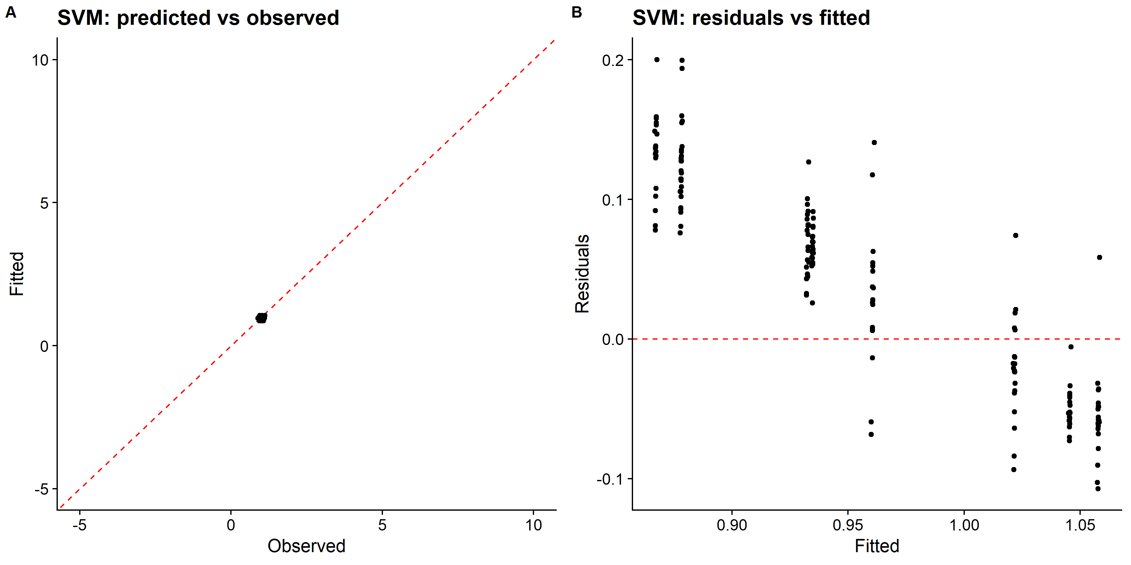

# looking at model performance
svm_perfomance <- svm_res %>% show_best(n = 1)
print(svm_perfomance) # rmse: 0.0492

## # A tibble: 1 x 9
##    cost margin .metric .estimator   mean     n std_err .config .iter
##   <dbl>  <dbl> <chr>   <chr>       <dbl> <int>   <dbl> <chr>   <int>
## 1  2.34 0.0955 rmse    standard   0.0846    25 0.00166 Iter5       5

The linear SVM model only predicted values of the standardized race time in a very small range, which looks like a single distinct value after rescaling, and the RMSE is the largest among all models so far. I should probably try other kernel SVM models such as polynomial or radical basis function that performs better for nonlinear decision boundary.

Null RMSE with standard error

# Calculate the null RMSE and SE by boostrapping
res <- numeric(1000)
for (i in 1:1000) {
  Bi <- as.numeric(unlist(train_data[sample(1:nrow(train_data), size = nrow(train_data), replace = TRUE), "std_time"]))
  res[i] <- rmse_vec(
    truth = Bi, estimate = rep(mean(train_data$std_time), nrow(train_data))
  )
}
null_rmse <- tibble(
  estimate = rmse_vec(truth = train_data$std_time,
                      estimate = rep(mean(train_data$std_time), nrow(train_data))),
  std_err = sd(res)
)

null_rmse  %>% 
  dplyr::mutate(across(everything(), ~round(.x, digits = 4))) %>% 
  knitr::kable(caption = "RMSE and boostrap SE (B = 1000) for the null model.")

RMSE and boostrap SE (B = 1000) for the null model.

estimate	std_err
0.0299	0.0026

tree_RMSE <- tree_res  %>%  
  show_best(n = 1) %>%  
  dplyr::select(estimate = mean, std_err) %>% 
  dplyr::bind_rows(null_rmse) %>% 
    dplyr::mutate(
    model = c("Tree", "Null"),
    rmse = round(estimate, 2),
    SE = round(std_err, 4),
    .keep = "unused"
  )

svm_RMSE <- svm_res  %>%  
  show_best(n = 1) %>%  
  dplyr::transmute(
    rmse = round(mean, 2),
    SE = round(std_err, 4),
    model = "SVM"
  ) %>%  
  dplyr::bind_rows(tree_RMSE)

rf_RMSE <- rf_res  %>%  
  show_best(n = 1) %>%  
  dplyr::transmute(
    rmse = round(mean, 2),
    SE = round(std_err, 4),
    model = "Random Forest"
  ) %>%  
  dplyr::bind_rows(svm_RMSE)

all_RMSE <- lasso_res  %>%  
  show_best(n = 1) %>%  
  dplyr::transmute(
    rmse = round(mean, 2),
    SE = round(std_err, 4),
    model = "LASSO"
  ) %>%  
  dplyr::bind_rows(rf_RMSE) %>% 
  gt::gt(caption = "Comparison of RMSE values for all models.")


all_RMSE

Comparison of RMSE values for all models.

rmse	SE	model
0.00	0.0000	LASSO
0.01	0.0005	Random Forest
0.08	0.0017	SVM
0.01	0.0005	Tree
0.03	0.0026	Null

# save RMSE comparison table 
rmse_location = here("tidytuesday2_figures", "rmsecomparison.Rds")
saveRDS(all_RMSE, file = rmse_location)

Model selection

We can see that LASSO had best fit compared to all other models. The predicted vs observed plot looks good, all the data points align well on the diagonal. So, I will fit the chosen LASSO model to the test data and evaluate the performance.

Final evaluation

# evaluate how model perform on test set
last_rf_fit <- final_lasso_wf %>% 
  last_fit(split = data_split, 
                 metrics = metric_set(rmse))

last_rf_fit %>% 
  collect_metrics()

## # A tibble: 1 x 4
##   .metric .estimator .estimate .config             
##   <chr>   <chr>          <dbl> <chr>               
## 1 rmse    standard    0.000757 Preprocessor1_Model1

# rmse for LASSO model fitting on testing data
lasso_test_rmse <- collect_metrics(last_rf_fit) %>% 
  dplyr::select(rmse = .estimate) %>% 
  dplyr::mutate(data = "testing")

# rmse for LASSO model fitting on training data  
lasso_RMSE_train <- lasso_res %>% 
  show_best(n = 1) %>% 
  dplyr::transmute(
    rmse = round(mean, 4),
    SE = round(std_err, 4),
    model = "LASSO"
  ) 

lasso_RMSE_train %>% 
  dplyr::transmute(
    rmse, data = "training"
  ) %>% 
  bind_rows(lasso_test_rmse) %>% 
  gt::gt(caption = "Comparison of RMSE between traing and testing data using LASSO regression.")

Comparison of RMSE between traing and testing data using LASSO regression.

rmse	data
0.0009000000	training
0.0007565904	testing

The result shows that the final LASSO model fits were similar between training and testing data.